A Conceptual View¶

This section presents a conceptual view, a mental model, of computing with the Cerebras architecture. Read this before you get into the details of how to write a kernel with CSL.

Important

The presentation in this section is highly simplified, meant only to provide a conceptual mental model. Many important details are omitted to focus on a few key high-level ideas on how to think of computing with the Cerebras architecture.

The Cerebras computation model uses a dataflow architecture. The Cerebras Wafer Scale Engine (WSE) contains hundreds of thousands of independent processing elements (PEs). All the PEs are implemented as a two-dimensional rectangular mesh on one single silicon wafer. See the following diagram showing the mesh of PEs.

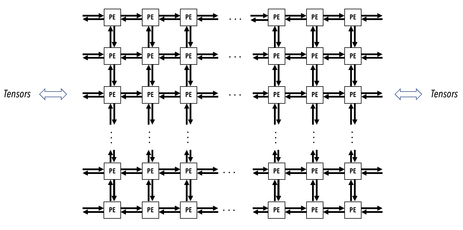
The operation of a Cerebras WSE can be described as follows: incoming data flows through the mesh of PEs. All the data that flows between the PEs does so in the form of 32-bit packet wavelets. As these wavelets flow through the mesh, they trigger transformations of the data. Hence the term dataflow computation model.

The mesh of interconnected PEs is called the fabric.

Fabric vs outside world

The fabric communicates the data to and from the outside world via parallel 100 Gigabit ethernet connections. These connections are also referred to as host I/O.

A processing element (PE)¶

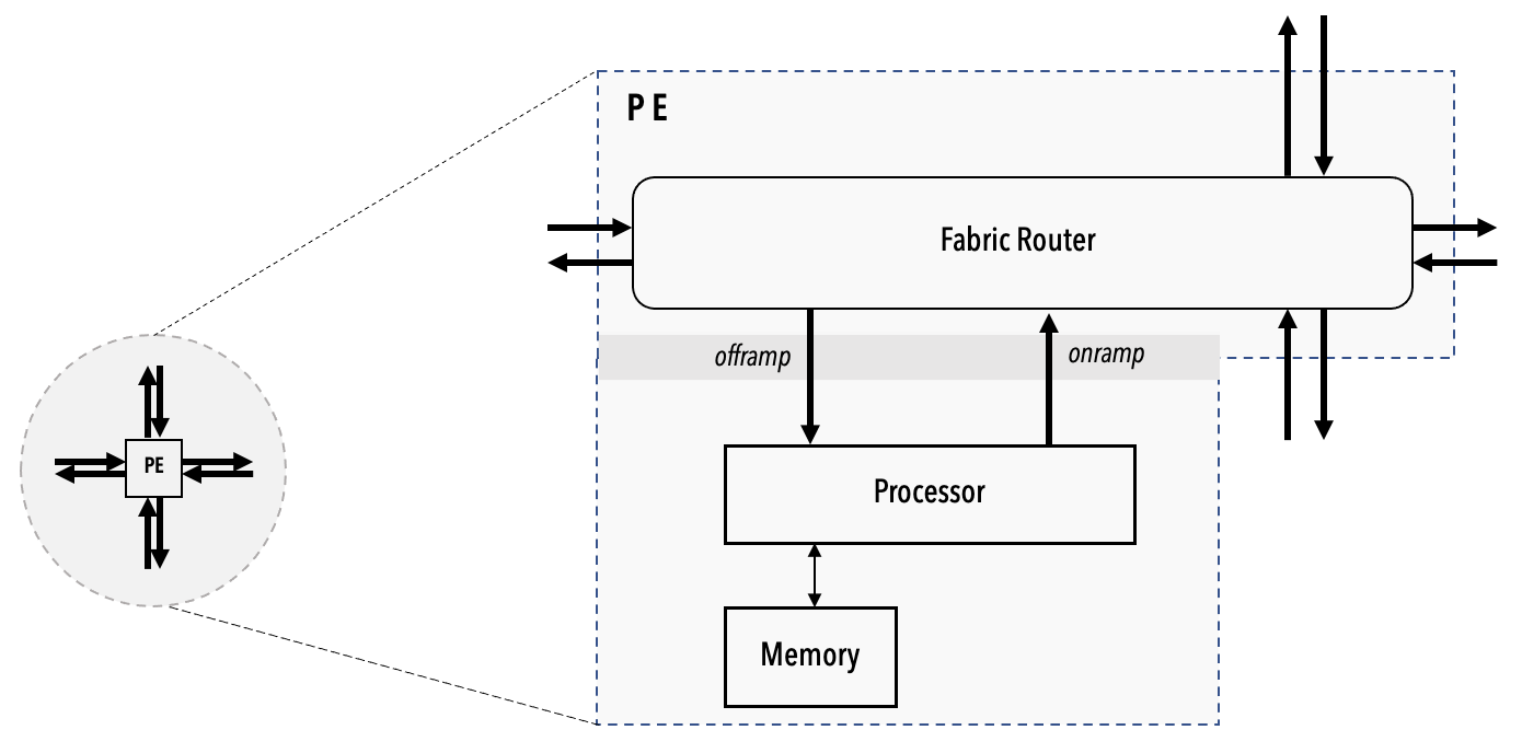
A PE is often also referred to as a tile. Each PE contains three key elements (see the following symbolic diagram):

A processor. Also referred as a compute engine (CE).
A router. Also referred as a fabric router. The router of a PE is directly connected via bidirectional links to its own CE and to the routers of the four nearest neighboring PEs in the mesh. The router is the only communication device the PEs use to send and receive data with other PEs.
The local tile memory. Each PE runs its own locally stored code. Neither the CE nor the local memory of a PE are directly accessible by other PEs.

The programming model¶

Developing your kernel for Cerebras WSE means you write your code in CSL, place the code in a file with a .csl extension, compile the code and use the Cerebras fabric simulator to test your code with inputs. When you are satisfied with your kernel performance with the fabric simulator, you can then target the actual network-attached WSE at your site.

CSL gives you full control of the WSE. To understand how to structure the kernel code in CSL, we need to comprehend a few key concepts first.

Task¶

A task defines the operations PEs perform. For example, a simple accumulation: result = result + data is a task. In CSL this is task is represented as:

task main_task(data: f16) void {
    result = result + data;
}

Rectangle¶

A Rectangle defines a contiguous group of PEs to perform a task. For example, two PEs could perform the above task. A program would define a Rectangle encompassing 1 x 2 PEs by specifying the coordinates and the (width, height) information. The following example shows how to set a Rectangle with width of 1 and a height of 2, i.e., a single column of two PEs in two rows, using the @set_rectangle() built-in function in CSL:

layout {
  @set_rectangle(1, 2);
  ...
}

Program PEs independently¶

You can program each PE in the fabric independently. You choose a Rectangle that contains either a single PE or a contiguous group of PEs. Only this Rectangle is aware of this task. Other Rectangles and other PEs in the fabric will be unaware of this task unless you explicitly also choose them for this task.

Bind wavelets to tasks¶

The basic way for a PE to operate on the data carried by a wavelet is to make the wavelet an input to the task.

Because you are able to program each Rectangle independently with its own set of input and output data, wavelets must be associated with specific tasks on your Rectangle. To accomplish this, you make use of the color of a wavelet and bind the wavelets you are interested in to the task.

In a dataflow architecture, the time when a task is executed depends on the time when the data inputs to it become available. This concept of input-data-triggered execution manifests in the notion of binding in Cerebras architecture.

Each wavelet has a 5-bit color tag. The color of a wavelet is how we distinguish one wavelet from another.

Note

The color of a wavelet is used in other ways, but the key idea is binding the color of a wavelet to a task. When you bind a wavelet color to a task, then when a wavelet of that color arrives at the PE, the task is triggered. We are omitting the important details of whether a task is blocked or unblocked, or whether the task is activated or inactive, but this is the basic idea of binding.

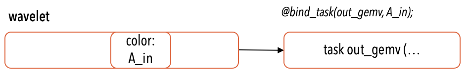
In your code you use the builtin CSL function @bind_task to create a binding between the color of the incoming wavelet and the task you want to execute. See the following conceptual diagram. The diagram shows a binding @bind_task(out_gemv, A_in) that indicates that the task out_gemv() will only be triggered in this specific Rectangle by the incoming wavelet of the specific color A_in.

See the following code example showing @bind_task in CSL:

// Define actions to perform at the start of the program execution
comptime {

    // Associate the appropriate task with the wavelet's color
    @bind_task(main_task, main_color);

    // Activate the color to run the task
    @activate(main_color);
}

Activating a task¶

Binding associates a task with a color on which data arrives in the form of wavelets. However, there is still the question of: “When does a task run?”. Conceptually, a task runs when it comes up in the order of execution and when all its inputs are available. When your CSL program is compiled, a task scheduler, working in the background, has determined the order of the execution of the task. But quite often a task can only be activated when all its inputs are available. Hence, the following applies:

By default tasks are unblocked and inactive. Simply creating a task will not be sufficient to activate it.
In order for a task to run it must be unblocked and active.

A task can be activated in at least two ways:

Using routable colors¶

You can simply bind the task to the wavelet color. When a wavelet on that color arrives, the task is activated and is run if the task is unblocked. You place the @bind_task() in the comptime block of your CSL program (we will cover comptime block and other CSL details elsewhere, but the syntax is simple, as shown below). Tasks such as these are wavelet-triggered tasks. Colors used in such wavelet-triggered tasks are routable colors.

comptime {
    ...
    @bind_task(main_task, main_color);
    ...
}

Using non-routable colors¶

You can explicitly activate the task by calling the builtin CSL function @activate() on the color that is bound to the task. You can place the @activate() function in the comptime block of your CSL program. This will make the task active at the start of the execution, i.e., the task runs at the start of the program execution similar to main() in other languages. See the example code below using the color my_nr_color.

When you activate a task in this explicit way, you are no longer letting the task sit inactive until a wavelet with my_nr_color color arrives, but instead you are triggering the task immediately upon the start of the program execution. For this reason, you must make sure that my_nr_color does not belong to any wavelet that is arriving through the fabric router into the PE. In other words, the color my_nr_color must not be a routable color, i.e., it must be a non-routable color. Tasks of the nature “startup tasks,” or “init tasks” are usually handled this way.

comptime {
    @bind_task(main_task, my_nr_color);
    @activate(my_nr_color);
}

Wavelets associated with the same color are all routed in the same way. Moreover, wavelets of the same color activate any and all tasks at any and all PEs as long as the task is bound to that color.

Layout¶

Layout is how you connect up the multiple PEs in your Rectangle in a way your computation requires. For example, see the following 2-PE Rectangle.

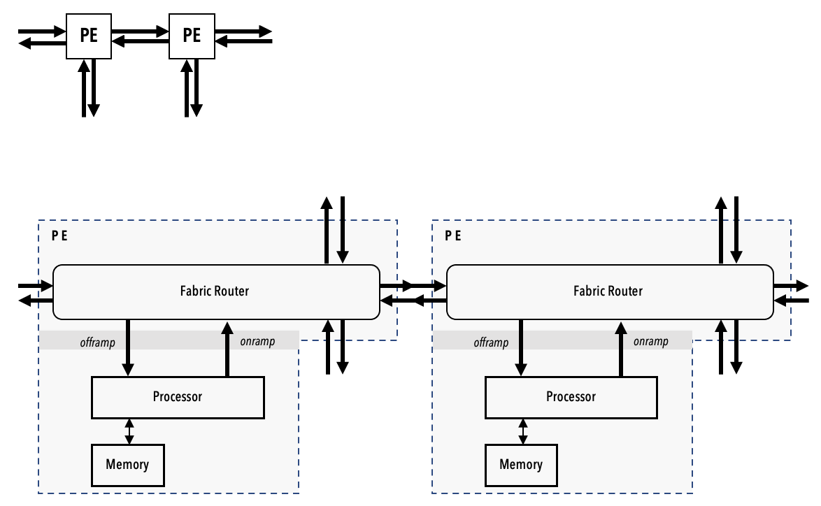
The diagram shows only one of the many ways you can interconnect the two PEs. You connect a PE to another PE by specifying routes and colors.

Using CSL you can define the specific colors and routes by which your Rectangle is stitched up. This configuration of colors and routes forms an essential aspect of your computation, transforming the wavelets as they enter and pass through your Rectangle after being processed by the task. See below an example of layout block showing a layout of two PEs in a single row:

// code.csl

// Top-level program source

const main_color: color = @get_color(0);

layout {
  @set_rectangle(2, 1); // A row containing two PEs.
  @set_tile_code(0, 0, "send.csl", .{ .send_color = main_color });
  @set_tile_code(1, 0, "recv.csl", .{ .recv_color = main_color });

  const send_route = .{ .rx = .{ RAMP }, .tx = .{ EAST } };
  const recv_route = .{ .rx = .{ WEST }, .tx = .{ RAMP } };

  @set_color_config(0, 0, main_color, send_route);
  @set_color_config(1, 0, main_color, recv_route);
}

The @set_tile_code() built-in CSL function is used to specify the .csl file containing the program for the individual PE. For example, the program “send.csl” contains the task description that only the PE at the coordinate (0, 0) will perform.

Note

Exactly one @set_rectangle() call is allowed. Zero or multiple calls are illegal.
The built-in @set_tile_code() must be called after calling the @set_rectangle().

For example, if your Rectangle contains five PEs, then you can configure each PE with a different program by having five @set_tile_code() calls after a single @set_rectangle(), with each @set_tile_code() function call specified with a separate .csl file.

Example¶

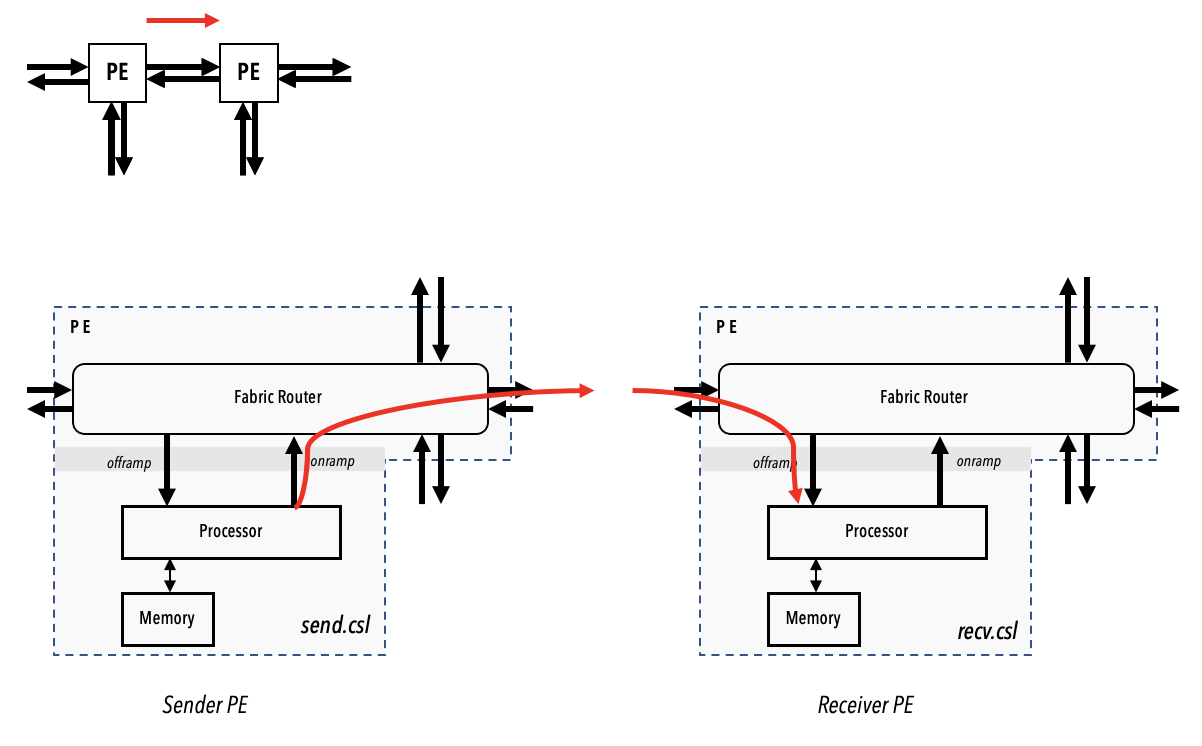
Exchange data between PEs¶

The following example program shows a Rectangle with two PEs. The PE on the left is configured to send a single 16-bit float value to the PE on the right.

Top-level program¶

Here is the top-level .csl program:

// Top-level program source

const main_color: color = @get_color(0);

layout {
  @set_rectangle(2, 1);
  @set_tile_code(0, 0, "send.csl", .{ .send_color = main_color });
  @set_tile_code(1, 0, "recv.csl", .{ .recv_color = main_color });

  const send_route = .{ .rx = .{ RAMP }, .tx = .{ EAST } };
  const recv_route = .{ .rx = .{ WEST }, .tx = .{ RAMP } };

  @set_color_config(0, 0, main_color, send_route);
  @set_color_config(1, 0, main_color, recv_route);
}

In the above top-level code, the @set_rectangle(2,1) on line 6 defines a single row of two PEs. The left PE is the sender, which routes wavelets from the ramp to east, and the right PE is the receiver, which routes wavelets from west to ramp. Both PEs use the same color, although they use different symbolic names for the same color value.

Sender¶

The following sender program sets up a memory data structure definition (DSD) to refer to the value to send, and uses the fabric DSD to send that value on the fabric.

// Sender program: send.csl

param send_color: color;

const src = [1]f16 { 42.0 };
const srcDsd = @get_dsd(mem1d_dsd, .{ .tensor_access = |i|{1} -> src[i] });

task send_task() void {
  const dstDsd = @get_dsd(fabout_dsd, .{.fabric_color = send_color, .extent = 1});
  @faddh(dstDsd, srcDsd, 0.0);
}

comptime {
  @bind_task(send_task, send_color);
}

Receiver¶

On the receiver side, the task simply updates the global variable with the wavelet data.

// Receiver program: recv.csl

param recv_color: color;
var result: f16 = 0.0;

task recv_task(wavelet_data: f16) void {
  result = wavelet_data;
}

comptime {
  @bind_task(recv_task, recv_color);
}

SDK Documentation (0.9.0)

A Conceptual View

Contents

A Conceptual View¶

A processing element (PE)¶

The programming model¶

Task¶

Rectangle¶

Program PEs independently¶

Bind wavelets to tasks¶

Activating a task¶

Using routable colors¶

Using non-routable colors¶

Layout¶

Example¶

Exchange data between PEs¶

Top-level program¶

Sender¶

Receiver¶